Insights · Passive Sensing & Detection

Multilateration Fundamentals: From Bearings and Time Differences to Tracks

September 2026 · 7 min read

AMBy Amardeep Mond, Founder & Chief Technology Officer, Aerodyne AI

A single passive sensor can tell you a direction, or a delay — never a position. A network of passive sensors can tell you where the target is, how fast it moves, and where it is going. The mathematics that performs this trick is over a century old: armies located enemy artillery by sound in the First World War using exactly the geometry described below. What has changed is not the math but the hardware — cheap sensors, cheap computing, and the need to find aircraft that emit nothing a receiver can range on.

Two kinds of passive measurement

A passive node — a microphone array, a radio receiver — fundamentally measures two things about a distant source. It can measure a bearing: the direction the sound or signal came from. And, paired with another node, it can measure a time difference of arrival (TDOA): the signal reached sensor A this much earlier than sensor B. Note what it cannot measure: the moment the signal left the target. An active radar knows that moment because it did the transmitting; a passive system, by definition, does not. Everything in passive localization is built from directions and differences, never from one-way absolute times — and that constraint shapes all the geometry that follows.

The geometry: hyperbolas, this time

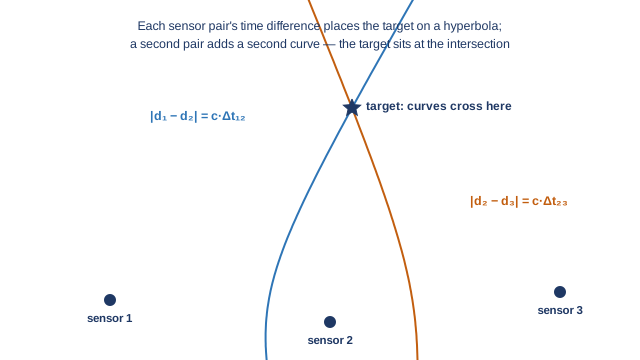
The previous article in this series showed that a bistatic radar's delay measurement places a target on an ellipse — the curve where the sum of two distances is constant. TDOA is the mirror image: the set of points where the difference of distances to two sensors is constant is a hyperbola with the two sensors at its foci. One pair of sensors gives one hyperbola; the target is somewhere along it. Add a third sensor and you get a second, independent hyperbola; the target sits where the curves cross. In three dimensions the same logic needs one more sensor, and the classical statistical treatment of exactly this problem — how measurement errors map into position errors for hyperbolic and bearing-based systems — has been standard reference material for decades [1].

Bearings compose even more simply: two sensors each report a direction, and the target sits where the two rays intersect — the surveyor's triangulation, unchanged since antiquity. Its error behavior, however, deserves a number. An angular error is a slice of arc, and arc length grows with range: a one-degree bearing error corresponds to roughly 17 meters of cross-range uncertainty at one kilometer, but 175 meters at ten. Bearing-only systems are therefore precise nearby and progressively vague with distance, which is one reason real networks mix bearing and timing measurements rather than relying on either alone.

GDOP: how geometry multiplies error

Here is the least intuitive and most consequential fact in localization: two networks with identical sensors can produce wildly different position accuracy, purely because of where the sensors stand. Picture two bearing rays crossing at nearly ninety degrees: their intersection is pinned inside a small, tidy box of uncertainty. Now picture the same two rays crossing at a grazing five degrees — as happens when the target lies far outside the sensor baseline: the intersection region stretches into a long, thin sliver, and a tiny wobble in either bearing slides the estimated position hundreds of meters along it. The satellite-navigation literature gave this effect its standard name — geometric dilution of precision, GDOP — and its standard formulation: a dimensionless multiplier, computed from geometry alone, that scales raw measurement error into position error [2]. GDOP near one means geometry is helping; GDOP of ten means the same sensors are delivering ten times worse fixes because of where they stand.

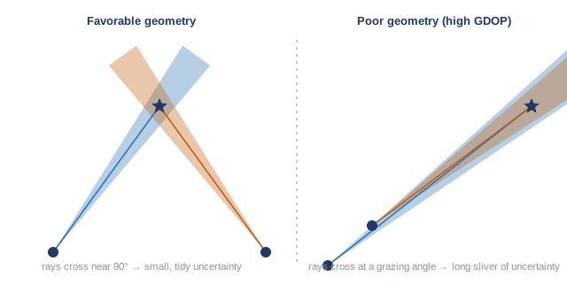
The design consequence is blunt: node placement is half the accuracy budget. A network laid out so that expected threat axes are seen from wide, crossing angles will outperform a "better" sensor deployed with poor geometry — and coverage planning for a passive network is, at bottom, the exercise of buying low GDOP over the ground you care about. It also yields the network's characteristic grace: losing one node does not blind the system; it degrades the geometry, raising GDOP over part of the map — a quantifiable, partial loss rather than a binary one.

The clock problem: why sound forgives and radio does not

TDOA has a hidden prerequisite: the sensors must agree on what time it is, to a precision matched to the signal's speed. The arithmetic is one line. Sound travels about 343 meters per second, so a one-millisecond clock disagreement corrupts an acoustic range difference by only 34 centimeters — audio networks can synchronize almost casually. Radio travels at the speed of light, 300 million meters per second, so the same one-millisecond error would be 300 kilometers of range error; RF multilateration demands agreement at the nanosecond scale, where one nanosecond equals 30 centimeters. The convenient engineering answer is disciplining every node's clock to satellite navigation signals — which immediately raises the contested-environment question, since satellite timing is jammable. A substantial published research literature exists on synchronizing distributed nodes wirelessly without satellite dependence; for the defender, the honest planning assumption is that timing is infrastructure, and like all infrastructure it must be designed for the day it is attacked.

From crossings to tracks

A single fix — one crossing of curves at one instant — is noisy and, with multiple simultaneous targets, ambiguous: many hyperbolas from many sources intersect in places where no aircraft is, producing ghost solutions. Both problems yield to time. Filtering a sequence of fixes through a motion model — the recursive estimation framework descending from Kalman's 1960 paper [3] — smooths noise, produces velocity as a byproduct, and discards ghosts, because ghost intersections do not move the way physical aircraft can. And one physical subtlety matters for acoustics specifically: sound is slow enough that the network localizes where the target was when it made the sound — a drone three kilometers away is heard roughly nine seconds late, in which time a fast platform has moved hundreds of meters. The fix is not a flaw but a modeling requirement: the tracker's motion model carries the delay and projects the target forward, which is routine once stated and wrong only when forgotten.

The architectural moral

Multilateration is the mathematics that converts many cheap, silent sensors into one instrument. Its accuracy is bought with geometry and timing rather than with transmitter power; its failure mode under node loss is gradual rather than total; and its output — tracks with velocity — is exactly the currency the fusion and engagement layers of a defense network consume, a hand-off this series takes up in the fusion article. None of this is proprietary insight. It is a century-old discipline, fully documented in the open literature, whose time has come back around because the targets stopped transmitting.

References

1. D. J. Torrieri, "Statistical theory of passive location systems," IEEE Transactions on Aerospace and Electronic Systems, vol. AES-20, no. 2, 1984.
2. E. D. Kaplan and C. J. Hegarty (eds.), Understanding GPS/GNSS: Principles and Applications, 3rd ed., Artech House, 2017.
3. R. E. Kalman, "A new approach to linear filtering and prediction problems," Journal of Basic Engineering, vol. 82, 1960.

This article synthesizes publicly available academic literature and public reporting. It describes concepts and results from the open published record and contains no Aerodyne technical data, system specifications, or performance information.